Lmoptimizebnd

From Eigenvector Documentation Wiki

Starting at (x0) LMOPTIMIZE finds (x) that minimizes the function defined by the function handle (fun) where (x) has parameters. Inputs (xlow) and (xup) can be used to provide lower and upper bounds on the solution (x). The function (fun) must supply the Jacobian and Hessian i.e. they are not estimated by LMOPTIMIZEBND (an example description is provided in the Algorithm Section of the function LMOPTIMIZE).

Inputs

fun = function handle, the call to fun is

[fval,jacobian,hessian] = fun(x)

[see the Algorithm section for tips on writing (fun)]

(fval) is a scalar objective function value,

(jacobian) is a x1 vector of Jacobian values, and

(hessian) is a x matrix of Hessian values.

x0 = x1 initial guess of the function parameters.
xlow = x1 vector of corresponding lower bounds on (x). See options.alow. If an element of xlow == -inf, the corresponding parameter in (x) is unbounded on the low side.
xup = x1 vector of corresponding upper bounds on (x). See options.aup. If an element of xup == inf, the corresponding parameter in (x) is unbounded on the high side.

Optional Inputs

options = discussed below in the Options Section.
params = comma separated list of additional parameters passed to the objective function (fun), the call to (fun) is

[fval,jacobian,hessian] = fun(x,params1,params2,...)

Outputs

x = x1 vector of parameter value(s) at the function minimum.
fval = scalar value of the function evaluated at (x).
exitflag = describes the exit condition with the following values

1: converged to a solution (x) based on one of the tolerance criteria

0: convergence terminated based on maximum iterations or maximum time.

out = structure array with the following fields:
critfinal: final values of the stopping criteria (see options.stopcrit above).
x: intermediate values of (x) if options.x=='on'.
fval: intermeidate values of (fval) if options.fval=='on'.
Jacobian: last evaluation of the Jacobian if options.Jacobian=='on'.
Hessian: last evaluation of the Hessian if options.Hessian=='on'.

Algorithm

The algorithm is essentially the same as that discussed in LMOPTIMIZE and this section discusses only the two main differences between LMOPTIMIZEBND and LMOPTIMIZE.

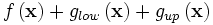
The first difference is the addition of penalty functions used to enforce bounding. For example, the objective function used in LMOPTIMIZE is $f\left( \mathbf{x} \right)$ , but the objective function used by LMOPTIMIZEBND is $f\left( \mathbf{x} \right)+g_{low}\left( \mathbf{x} \right)+g_{up}\left( \mathbf{x} \right)$ . The penalty functions for upper, $g_{up}\left( \mathbf{x} \right)$ , and lower bounds, $g_{low}\left( \mathbf{x} \right)$ , are similar, so only the lower penalty function is described.

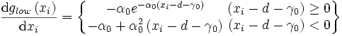
Define d as the lower boundary, $γ 0$ a small number (e.g. 0.001) and $α 0$ a large number [e.g. $- ln(10 - 8) / γ 0$ ], then for a single parameter the lower penalty function is given as

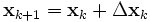
$g_{low}\left( x_{i} \right)=\left\{ \begin{matrix} e^{-\alpha _{0}\left( x_{i}-d-\gamma _{0} \right)} \\ 1-\alpha _{0}\left( x_{i}-d-\gamma _{0} \right)+\tfrac{1}{2}\alpha _{0}^{2}\left( x_{i}-d-\gamma _{0} \right)^{2} \\ \end{matrix}\text{ }\begin{matrix} \left( x_{i}-d-\gamma _{0} \right)\ge 0 \\ \left( x_{i}-d-\gamma _{0} \right)<0 \\ \end{matrix} \right\}$ .

This function can be considered an external point function because it is defined outside the feasible region (outside the boundaries). It is continuous at the boundary and also has continuous first and second derivatives. This is in contrast to internal point functions such as a log function that is not continuous at the boundary [e.g. ln(0) is not continuous]. The first and second derivatives of the penalty function are given by

$\frac{\text{d}g_{low}\left( x_{i} \right)}{\text{d}x_{i}}=\left\{ \begin{matrix} -\alpha _{0}e^{-\alpha _{0}\left( x_{i}-d-\gamma _{0} \right)} \\ -\alpha _{0}+\alpha _{0}^{2}\left( x_{i}-d-\gamma _{0} \right) \\ \end{matrix}\text{ }\begin{matrix} \left( x_{i}-d-\gamma _{0} \right)\ge 0 \\ \left( x_{i}-d-\gamma _{0} \right)<0 \\ \end{matrix} \right\}$ and

$\frac{\text{d}^{\text{2}}g_{low}\left( x_{i} \right)}{\text{d}x_{i}^{2}}=\left\{ \begin{matrix} \alpha _{0}^{2}e^{-\alpha _{0}\left( x_{i}-d-\gamma _{0} \right)} \\ \alpha _{0}^{2} \\ \end{matrix}\text{ }\begin{matrix} \left( x_{i}-d-\gamma _{0} \right)\ge 0 \\ \left( x_{i}-d-\gamma _{0} \right)<0 \\ \end{matrix} \right\}$ .

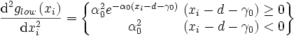The external point penalty function does not guarantee that a step won't move outside the boundaries into the infeasible region. It does, however provide a means for getting back inside the feasible region.

A second modification is included in the LMOPTIMIZEBND algorithm to avoid large steps outside the feasible region. If a step $\Delta \mathbf{x}_{k}$ is such that any $\mathbf{x}_{k+1}=\mathbf{x}_{k}+\Delta \mathbf{x}_{k}$ are outside the feasible region, the step size for those parameters is reduced. The reduction is 90% the distance of that parameter to the boundary. This typically changes the direction of the step $\Delta \mathbf{x}_{k}$ .

Options

options = structure array with the following fields:

display: [ 'off' | {'on'} ] governs level of display to the command window.
dispfreq: N, displays results every N^th iteration {default N=10}.
stopcrit: [1e-6 1e-6 10000 3600] defines the stopping criteria as [(relative tolerance) (absolute tolerance) (maximum number of iterations) (maximum time in seconds)].
x: [ {'off'} | 'on' ] saves (x) at each step.
fval: [ {'off'} | 'on' ] saves (fval) at each step.
Jacobian: [ {'off'} | 'on' ] saves last evaluation of the Jacobian.
Hessian: [ {'off'} | 'on' ] saves last evaluation of the Hessian.
ncond = 1e6, maximum condition number for the Hessian (see Algorithm).
lamb = [0.01 0.7 1.5], 3-element vector used for damping factor control (see Algorithm Section):

lamb(1): lamb(1) times the biggest eigenvalue of the Hessian is added to Hessian eigenvalues when taking the inverse; the result is damping.

lamb(2): lamb(1) = lamb(1)/lamb(2) causes deceleration in line search.

lamb(3): lamb(1) = lamb(1)/lamb(3) causes acceleration in line search.

ramb = [1e-4 0.5 1e-6], 3-element vector used to control the line search (see Algorithm Section):

ramb(1): if fullstep < ramb(1)\*[linear step] back up (start line search).

ramb(2): if fullstep > ramb(2)\*[linear step], accelerate [change lamb(1) by the acceleration parameter lamb(3)].

ramb(3): if linesearch rejected, make a small movement in direction of L-M step ramb(3)\*[L-M step].

kmax = 50, maximum steps in line search (see Algorithm Section).
alow: [ ], x1 vector of penalty weights for lower bound, {default = ones(N,1)}. If an element is zero, the corresponding parameter in (x) is not bounded on the low side.
aup: [ ], x1 vector of penalty weights for upper bound, {default = ones(N,1)}. If an element is zero, the corresponding parameter in (x) is not bounded on the high side.

Examples

options   = lmoptimize('options');
options.x = 'on';
options.display = 'off';
options.alow    = [0 0]; %x(1) and x(2) unbounded on low side
options.aup     = [1 0]; %x(1) bounded on high side and x(2)
                         % unbounded on high side

[x,fval,exitflag,out] = lmoptimize(@banana,x0,[0 0], ...
                          [0.9 0],options);
plot(out.x(:,1),out.x(:,2),'-o','color', ...
 [0.4 0.7 0.4],'markersize',2,'markerfacecolor', ...
 [0 0.5 0],'markeredgecolor',[0 0.5 0])

Lmoptimizebnd

From Eigenvector Documentation Wiki

Contents

Purpose

Synopsis

Description

Inputs

Optional Inputs

Outputs

Algorithm

Options

Examples

See Also

Views

Personal tools

Navigation